Sunday, April 27, 2008
WG Grace
WG Grace had a very long career — he played a long time after his peak. That's why, when looking at his career averages (unadjusted first-class averages from CricketArchive: bat 39,45; bowl 18,14), you don't see why he's such a huge figure in the history of the game. His aggregates are huge, sure, but it looks like he was a great who played for a long time, rather than a rival to Bradman as the greatest ever.
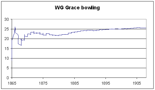
To see where this latter perception comes from, I plotted his cumulative adjusted averages (weighting innings according to the quality of the attack, relative to an overall average of 24,5) against time. I considered only first-class matches in England (since I know that that part of my database works — I didn't want to spend half a week debugging Australian matches that I haven't tested yet).
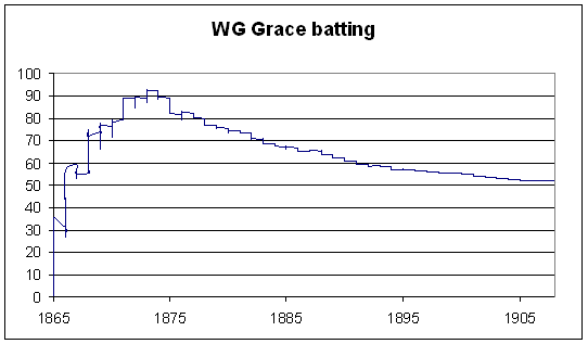
To give a feel for the batting scale: Bradman is at 98,9; Headley 65,8; Ranji 60,5; Merchant 56,3 (those are the top four); Mike Hussey 52,2; Barry Richards 45,3.
Bowling scale: Murali 13,7; Lindwall 14,1 (top two); Darren Gough 20,9; Eddie Hemmings 25,6.
All references to averages below are adjusted ones.
Grace's (adjusted) batting average peaked at the end of the 1873 season at 92,8; at this time he had scored over 10000 first-class runs. Batting doesn't get much more Bradmanesque. By 1880, he had 19560 runs at 74,5. This also marks the start of his decline as a bowler. By the end of 1880, he had 1335 wickets at 21,9. If Grace had stopped playing then, his ratio of batting average to bowling average (3,4) would have been well clear of second place (Keith Miller at 2,8).
Even in 1886, though (more than 20 years after the start of his first-class career), his batting average was higher than Headley's.
The decline in batting average is very marked — it almost falls to 50 by the end of his career. The rise in his bowling average is much more gentle, because as he got older he bowled less, not bowling more than 4000 balls in a season after 1888.
To see where this latter perception comes from, I plotted his cumulative adjusted averages (weighting innings according to the quality of the attack, relative to an overall average of 24,5) against time. I considered only first-class matches in England (since I know that that part of my database works — I didn't want to spend half a week debugging Australian matches that I haven't tested yet).


To give a feel for the batting scale: Bradman is at 98,9; Headley 65,8; Ranji 60,5; Merchant 56,3 (those are the top four); Mike Hussey 52,2; Barry Richards 45,3.
Bowling scale: Murali 13,7; Lindwall 14,1 (top two); Darren Gough 20,9; Eddie Hemmings 25,6.
All references to averages below are adjusted ones.
Grace's (adjusted) batting average peaked at the end of the 1873 season at 92,8; at this time he had scored over 10000 first-class runs. Batting doesn't get much more Bradmanesque. By 1880, he had 19560 runs at 74,5. This also marks the start of his decline as a bowler. By the end of 1880, he had 1335 wickets at 21,9. If Grace had stopped playing then, his ratio of batting average to bowling average (3,4) would have been well clear of second place (Keith Miller at 2,8).
Even in 1886, though (more than 20 years after the start of his first-class career), his batting average was higher than Headley's.
The decline in batting average is very marked — it almost falls to 50 by the end of his career. The rise in his bowling average is much more gentle, because as he got older he bowled less, not bowling more than 4000 balls in a season after 1888.
Saturday, April 26, 2008
Bowler workloads
Over at CFF, there was a debate over spinners' averages. One poster said that spinners bowl disproportionately many overs on flat pitches, while lazy pacemen rotate at the other end. This has the effect of bloating out spinners' averages unfairly. Another poster responded by saying that spinners also bowl disproportionately many overs on raging turners, which would help their averages.
Which factor is the dominant one? To answer this, I considered every innings, and scaled each bowlers' figures so that he effectively bowled a quarter of the overs. So, for instance, if a team batted for 100 overs, and one bowler took 1/80 from 20 overs, that would be scaled up to 1,25/100 from 25 overs. If another bowler took 1/60 from 30, it would become 0,83/50. So each bowler's average in any given innings won't change, but we'll see any effects of bowling or not bowling in tough or easy conditions.
Now, sometimes a bowler might, say, bowl one over in an innings and take a wicket in it, or bowl one over and get hit for 15 runs. Obviously it's not realistic that he would have taken 25 wickets or gone for 375 runs from 25 overs, so if the number of balls bowled by a bowler was less than 60, I didn't do any adjustment. It's a bit arbitrary where you put the cut-off, but pushing it back to 30 balls doesn't change the overall trends.
One very stunning result comes out of this analysis. Every major wicket-taker (at least 100 Test wickets), except for Vanburn Holder, has his average increase. I'm still wondering a little bit if it's a bug in my code, but since I can't find one, and it passes various sanity checks, I'm reasonably confident that these results are true.
Assuming that I haven't made some silly mistake, there's a simple explanation for this phenomenon — captains can tell which bowlers are being effective on a given day and which ones aren't, and they make the effective bowlers bowl more overs. There could also be a bit of luck involved — say a bowler is a bit unlucky and goes for fifteen wicketless overs. If he'd been given another ten, he might have picked up a wicket or two. But since he hadn't, he didn't get to bowl again.
Let's have a look at the top and bottom of the table, ordered by the difference in weighted (by the average of the batsmen dismissed) average. Qualification: 100 wickets. Columns of the table are: wickets, regular average, weighted average, scaled regular average, scaled weighted average, difference between scaled regular average and regular average, difference between scaled weighted average and weighted average.
Those near the top of the table are the ones who bowl in the tough conditions or don't bowl so often in favourable ones; those near the bottom don't bowl so much in the tough conditions but do when things are going well.
The results aren't what I would have expected. Murali's position near the top is easy to explain — he does a huge amount of bowling for Sri Lanka come what may. Generally, though, it's pacemen at the top and spinners at the bottom.
The keen-eyed amongst you will note that, with the exception of Murali, none of the bowlers listed above took more than 155 wickets. There is much more variation for bowlers with lower numbers of wickets:
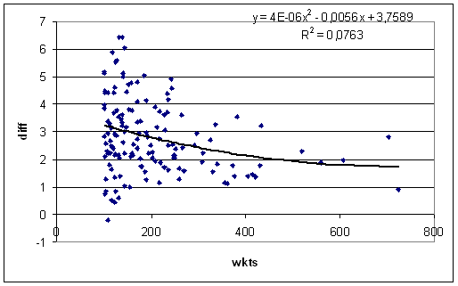
I've shown a quadratic fit because it looks better than a linear one. The general trend is clearly downward — bowlers who take lots of wickets tend to get hidden less from flat pitches than bowlers who don't.
Now of course, considering only bowlers with large career wicket hauls will pick out good bowlers, but what about great bowlers from the olden days who didn't play so many Tests? If you take the ratio of scaled weighted average to weighted average, and plot against the weighted average, you get only a very very slight positive correlation (y = 0,0008x + 1,07; R-squared = 0,01).
(If you plot the difference, rather than the ratio, you get a strong positive correlation. I think it's more accurate to work with ratios here.)
So, my conclusions so far are:
- Most of the variation is to do with small samples.
- But better bowlers do have slightly smaller differences (or ratios) when you scale their workloads to one quarter of each innings' overs.
Murali definitely belongs near the top of the table — such a small difference after taking over 700 wickets is clearly a genuine (and easily explained) trait of his bowling, and not statistical noise. This looks to me like a good way of trying to answer the question, "How would Warne have done if he had Murali's workload?" I don't think it's reasonable to do this for most pairs of bowlers, but if they have a large number of wickets (as with Warne and Murali), then the difference between a pair of players is likely to be genuine. And in this case, Murali comes out easily the better.
Now to the question that started this all — spinners v pacemen. For pacemen, the average ratio of scaled weighted average to weighted average is 1,08. For spinners it's 1,11. So it looks like spinners getting to bowl on raging turners is a bigger factor for their averages than having to shoulder the workload on flat tracks. Doing the diff v wkts plot as above for spinners and quicks separately clearly shows the quicks (on average) having smaller differences across all lengths of career.
Lastly, if you only scale downwards (i.e., if they bowled more than a quarter of the overs, then scale back to a quarter, else do nothing), then the ratios become 1,05 for quicks and 1,08 for spinners.
Which factor is the dominant one? To answer this, I considered every innings, and scaled each bowlers' figures so that he effectively bowled a quarter of the overs. So, for instance, if a team batted for 100 overs, and one bowler took 1/80 from 20 overs, that would be scaled up to 1,25/100 from 25 overs. If another bowler took 1/60 from 30, it would become 0,83/50. So each bowler's average in any given innings won't change, but we'll see any effects of bowling or not bowling in tough or easy conditions.
Now, sometimes a bowler might, say, bowl one over in an innings and take a wicket in it, or bowl one over and get hit for 15 runs. Obviously it's not realistic that he would have taken 25 wickets or gone for 375 runs from 25 overs, so if the number of balls bowled by a bowler was less than 60, I didn't do any adjustment. It's a bit arbitrary where you put the cut-off, but pushing it back to 30 balls doesn't change the overall trends.
One very stunning result comes out of this analysis. Every major wicket-taker (at least 100 Test wickets), except for Vanburn Holder, has his average increase. I'm still wondering a little bit if it's a bug in my code, but since I can't find one, and it passes various sanity checks, I'm reasonably confident that these results are true.
Assuming that I haven't made some silly mistake, there's a simple explanation for this phenomenon — captains can tell which bowlers are being effective on a given day and which ones aren't, and they make the effective bowlers bowl more overs. There could also be a bit of luck involved — say a bowler is a bit unlucky and goes for fifteen wicketless overs. If he'd been given another ten, he might have picked up a wicket or two. But since he hadn't, he didn't get to bowl again.
Let's have a look at the top and bottom of the table, ordered by the difference in weighted (by the average of the batsmen dismissed) average. Qualification: 100 wickets. Columns of the table are: wickets, regular average, weighted average, scaled regular average, scaled weighted average, difference between scaled regular average and regular average, difference between scaled weighted average and weighted average.
                          avg      scaled avg    diff
name             wkts  reg   wtd   reg   wtd   reg   wtd
VA Holder        109   33,3  37,0  33,1  36,8  -0,2  -0,2
DA Allen         122   31,0  30,1  32,4  30,6  1,4   0,4
PM Pollock       116   24,2  26,5  24,9  27,0  0,7   0,5
M Dillon         131   33,6  31,4  34,3  32,1  0,7   0,6
AN Connolly      102   29,2  27,1  29,3  27,9  0,0   0,7
CEH Croft        125   23,3  23,3  24,3  24,1  1,0   0,8
NAT Adcock       104   21,1  23,5  22,1  24,3  1,0   0,9
M Muralitharan   724   21,8  24,6  22,5  25,5  0,6   0,9
MW Tate          155   26,2  26,3  26,9  27,3  0,8   1,0
WJ O'Reilly      144   22,6  22,8  23,1  23,8  0,5   1,0
---
C Blythe         100   18,6  23,8  22,5  28,9  3,9   5,1
H Trumble        141   21,8  26,5  25,8  31,6  4,0   5,1
Mohammad Rafique 100   40,8  40,6  45,4  45,8  4,7   5,2
N Boje           100   42,7  38,9  48,4  44,0  5,8   5,2
Intikhab Alam    125   36,0  37,4  41,8  42,9  5,8   5,5
W Rhodes         127   27,0  32,7  31,4  38,3  4,4   5,6
J Briggs         118   17,8  32,4  21,9  38,3  4,1   5,9
AF Giles         143   40,6  37,7  46,9  43,7  6,3   6,0
TE Bailey        132   29,2  30,6  35,6  37,1  6,4   6,4
AL Valentine     139   30,3  33,2  35,9  39,6  5,6   6,4
Those near the top of the table are the ones who bowl in the tough conditions or don't bowl so often in favourable ones; those near the bottom don't bowl so much in the tough conditions but do when things are going well.
The results aren't what I would have expected. Murali's position near the top is easy to explain — he does a huge amount of bowling for Sri Lanka come what may. Generally, though, it's pacemen at the top and spinners at the bottom.
The keen-eyed amongst you will note that, with the exception of Murali, none of the bowlers listed above took more than 155 wickets. There is much more variation for bowlers with lower numbers of wickets:

I've shown a quadratic fit because it looks better than a linear one. The general trend is clearly downward — bowlers who take lots of wickets tend to get hidden less from flat pitches than bowlers who don't.
Now of course, considering only bowlers with large career wicket hauls will pick out good bowlers, but what about great bowlers from the olden days who didn't play so many Tests? If you take the ratio of scaled weighted average to weighted average, and plot against the weighted average, you get only a very very slight positive correlation (y = 0,0008x + 1,07; R-squared = 0,01).
(If you plot the difference, rather than the ratio, you get a strong positive correlation. I think it's more accurate to work with ratios here.)
So, my conclusions so far are:
- Most of the variation is to do with small samples.
- But better bowlers do have slightly smaller differences (or ratios) when you scale their workloads to one quarter of each innings' overs.
Murali definitely belongs near the top of the table — such a small difference after taking over 700 wickets is clearly a genuine (and easily explained) trait of his bowling, and not statistical noise. This looks to me like a good way of trying to answer the question, "How would Warne have done if he had Murali's workload?" I don't think it's reasonable to do this for most pairs of bowlers, but if they have a large number of wickets (as with Warne and Murali), then the difference between a pair of players is likely to be genuine. And in this case, Murali comes out easily the better.
               wtd avg   sc wtd avg
M Muralidaran  24,6      25,5
SK Warne       27,9      30,7
Now to the question that started this all — spinners v pacemen. For pacemen, the average ratio of scaled weighted average to weighted average is 1,08. For spinners it's 1,11. So it looks like spinners getting to bowl on raging turners is a bigger factor for their averages than having to shoulder the workload on flat tracks. Doing the diff v wkts plot as above for spinners and quicks separately clearly shows the quicks (on average) having smaller differences across all lengths of career.
Lastly, if you only scale downwards (i.e., if they bowled more than a quarter of the overs, then scale back to a quarter, else do nothing), then the ratios become 1,05 for quicks and 1,08 for spinners.
Tuesday, April 22, 2008
More on getting your eye in
I've left things too late for a comprehensive post, but since I'm disappearing again for a few days (Toulouse and Carcassonne this time), I thought I'd do a little post on those effective average curves without coming to any sweeping conclusions.
Some of the fits seem to have fallen into a local minimum that doesn't describe the effective average curve very well. Most obvious of these is Mark Richardson, who apparently always bats like he averages 57 but really only averages 45 (eyeballing his empirical hazard function, I think his effective average starts high and decreases). Such clearly wrong curves seem to be pretty rare, so hopefully they don't poison the overall trends too much.
Best and worst on nought (qualifications: average of 35, and some minimum number of innings, probably 50):
But as I said in my previous post, much of the variation in how players do on nought can be put down to chance. Not all of it, though, so some of those names in the table above should belong around where you see them.
Here's a plot of effective average at nought against regular average:

Now the effective average on 1 against regular average (there's much less scatter because there's basically no smoothing done at nought, but there is at 1):

Effective average at 10:

Effective average at 30:

The effective average at 10 is very good at predicting the overall average — the scatter is noticeably less than at 1 or 30 (I haven't tried numbers in between to see where the minimum actually is). Part of this might be an artefact of the model, but I think that part of this is a real effect, especially the larger scatter at 30. Good players should have their eye in by 30 and do much better than their overall average. Bad players don't improve so much from how they did earlier in their innings. Why don't they improve? Why do they get as much eye in as possible (which is not very much) early in their innings? Questions for psychologists perhaps.
Some of the fits seem to have fallen into a local minimum that doesn't describe the effective average curve very well. Most obvious of these is Mark Richardson, who apparently always bats like he averages 57 but really only averages 45 (eyeballing his empirical hazard function, I think his effective average starts high and decreases). Such clearly wrong curves seem to be pretty rare, so hopefully they don't poison the overall trends too much.
Best and worst on nought (qualifications: average of 35, and some minimum number of innings, probably 50):
name          µ(0)  µ(1)  µ(10) µ(30) avg
MH Richardson 57,4  57,4  57,4  57,4  44,8
AN Cook       53,3  49,5  46,5  44,3  43,5
AL Hassett    52,1  52,1  52,1  48,0  46,6
CL Walcott    47,1  47,2  50,1  62,8  56,7
CH Lloyd      42,6  46,7  47,7  48,3  46,7
H Sutcliffe   41,0  73,8  75,0  75,6  60,7
Saeed Ahmed   39,1  41,3  41,3  41,3  40,4
CC McDonald   36,8  41,1  41,1  41,1  39,3
PE Richardson 35,8  36,8  36,8  36,8  37,5
GM Ritchie    35,8  16,9  33,4  34,9  35,2
---
DL Amiss      7,8   29,4  39,6  46,2  46,3
NS Sidhu      7,7   37,0  46,8  52,6  42,1
MW Gatting    7,6   26,2  37,1  44,4  35,6
VL Manjrekar  7,4   42,5  42,5  42,5  39,1
DM Jones      7,1   35,7  46,1  52,2  46,6
FMM Worrell   6,9   37,6  51,5  60,2  49,5
JA Rudolph    6,9   23,0  33,9  41,4  36,2
FE Woolley    6,5   41,1  44,3  46,0  36,1
CG Borde      6,5   36,7  41,1  43,5  35,6
MS Atapattu   6,1   32,5  36,4  38,4  39,0
But as I said in my previous post, much of the variation in how players do on nought can be put down to chance. Not all of it, though, so some of those names in the table above should belong around where you see them.
Here's a plot of effective average at nought against regular average:

Now the effective average on 1 against regular average (there's much less scatter because there's basically no smoothing done at nought, but there is at 1):

Effective average at 10:

Effective average at 30:

The effective average at 10 is very good at predicting the overall average — the scatter is noticeably less than at 1 or 30 (I haven't tried numbers in between to see where the minimum actually is). Part of this might be an artefact of the model, but I think that part of this is a real effect, especially the larger scatter at 30. Good players should have their eye in by 30 and do much better than their overall average. Bad players don't improve so much from how they did earlier in their innings. Why don't they improve? Why do they get as much eye in as possible (which is not very much) early in their innings? Questions for psychologists perhaps.
Monday, April 14, 2008
London trip
Tomorrow I'll be heading to London, where I'll be until the end of the week. For the first time in almost a year, I'll actually watch a day of cricket. I don't mean that I haven't been to a cricket ground for a year (it's been longer than that) — I'm including television as well. It's been a while. So let's hope that the rains stay away on Wednesday for the first day of the Championship, and in particular Surrey v Lancashire.
So before I disappear for a week, here's a quick run-down on what I've done on getting your eye in in the last couple of days. I worked out how to script gretl, so I've now got effective average curves for pretty much all major batsmen (there are a few with really bizarre hazard functions that refused have my curve type fitted to them).
There doesn't appear to be any substantial differences in effective average on nought between openers, all-rounders, and others.
All-rounders might behave differently in terms of how they perform once they're off the mark, but I need to have a bit of a more careful look.
I'm wondering how much of the variation in effective average on nought is due to luck. Looking at batsmen who average over 40, the average proportion of ducks is about 0,061. Using that and applying the binomial theorem with 120 innings (the average number of innings across the dataset), you get an expected standard deviation of 0,022. The actual standard deviation is 0,024. About 60% are within one standard deviation of the mean, a little less than would be predicted (68,7%) by the normal distribution. (I'm assuming there's enough innings for the normal distribution to be a good approximation.) So it looks like there are real differences between batsmen in terms of ducks, but they might not be so big.
Friday, April 11, 2008
Getting your eye in
(Update: See these two followup posts.)
An anonymous commenter pointed me to arXiv:0801.4408v1, a paper by Brendon Brewer called "Getting Your Eye In: A Bayesian Analysis of Early Dismissals in Cricket".
Before starting the discussion, I'll define the hazard function. These seem to be used all over the place in the (pretty small) academic literature on cricket scores. The hazard function, written H(x), is defined as the probability that the batsman will be dismissed at score x.
Simple enough. But Brewer points out a very neat interpretation of it (he may not be the first to do so, but it's the first time I've seen it). If the hazard function is constant (i.e., always equal probability of getting out), you get a geometric distribution of scores (or, in the continuous limit, the exponential distribution that I mention every couple of weeks). In particular, a hazard value H is related to a batting average µ by µ = 1/H - 1.
So (here's the important bit), given a particular value of H for some batsman (say H(0) = 0,06 — the probability of making a duck), we can say that, on zero, he bats like someone with an average of 1/0,06 - 1 = 15,67. If you're not convinced that this is useful, you should be by the end of this post.
Technical details follow. Feel free to skip to the tables below.
The methods used in the paper are too technical for me to be bothered understanding them all, but here is a brief summary:
- Assume that the hazard function is of a particular type depending on various parameters.
- Estimate what those parameters are.
I think that the main problem with the assumptions is that they don't take into account how important getting off the mark is. It's assumed that it's a pretty smooth transition from zero to some higher score. But, if you work out the hazard directly (I took all batsmen who average over 40 in Tests), you get this:
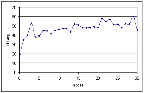
There's an almost 20-run jump in effective average from a score of zero to a score of one. (Also, it curve doesn't level off for a long time.)
So, I instead took assumed that the average associated with the hazard goes like:
µ = a + k*(b - a)*xp.
I originally intended for all of those parameters to have nice interpretations, but the actual results made a mockery of that idea. Anyway, if you fit the graph above up to x = 30, you get the following (fit parameters: a = 15,2; b = 49,4; k = 0,63; p = 0,17):
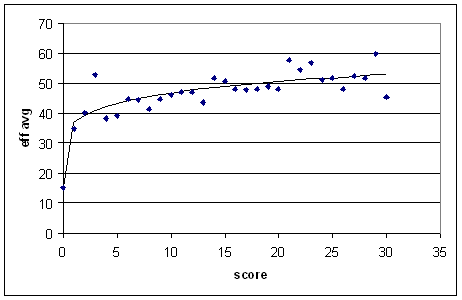
Technical notes: I did the fits using gretl's non-linear least squares abilities. You do the fits with the hazard function and then convert to an average, since sometimes the hazard function gets close to or equal to zero. If you convert to an average before fitting, you get some data points heading off to infinity and nothing works. I used scores from 0 to 49. The way the equation's set up, the parameter 'a' basically picks out the empirical hazard at zero. I think that this is reasonable, since getting off the mark is so important. But it's debatable.
Unfortunately, I don't know how to automate everything, so I have to do one batsman at a time. Maybe next time I'm listening to football on the radio I'll go through and process a bunch of batsmen.
Now, the parameter 'a' does have a nice interpretation: it's the effective batting average at zero. The parameter 'p' tells you how flat the curve is (near zero: very flat). While I give the values of the parameters for each player, the more important thing is the effective average µ at various scores. I've given µ(0) (which is just 'a'), µ(1) (effective average at 1), µ(10), and µ(30). There's a bit of round-off error (I went gretl -> pen and paper -> Excel), but it's nothing serious. I've also given the regular average in the last column.
To start with, here's the very atypical example of Don Bradman:
Don't let Bradman get off the mark! On zero he batted like someone who averaged 10, but on one he was almost as good as Mike Hussey. Very soon he batted like the best batsmen ever. Bradman's apparent woefulness before he got off the mark seems pretty typical. Let's have a look at some others.
Interestingly, the two best batsmen on nought are Langer and Kirsten — both openers. Unfortunately, this is a (very) limited dataset, so we'll put this aside for further study.
In Brewer's own small dataset, he saw that the two all-rounders had little change from "before eye in" to "eye in". Part of that I think is due to the wrong shape of the hazard function, but all-rounders doing well on nought does seem to be a real effect (again, pending a more thorough study):
In terms of flatness of the effective average (once off the mark), I think the most important factor is the regular average. Sorta-all-right batsmen who average 30 will typically get lots of starts but not go on with them. Two examples (again it'd be nice to have more, but I didn't cherrypick — they were the only two I looked at):
So players like Ramprakash and Mahanama have got their eye in once they're off the mark, but that's as far as it goes. Better batsmen continue to improve, but these ones don't, for whatever reasons.
That's all I have for now. Feel free to make requests, and to make it interesting, say what you think the results will be for each batsman (e.g., terrible on zero, good on zero, etc.).
And I hope you're all convinced that the effective average is a wonderful number for this exercise.
An anonymous commenter pointed me to arXiv:0801.4408v1, a paper by Brendon Brewer called "Getting Your Eye In: A Bayesian Analysis of Early Dismissals in Cricket".
Before starting the discussion, I'll define the hazard function. These seem to be used all over the place in the (pretty small) academic literature on cricket scores. The hazard function, written H(x), is defined as the probability that the batsman will be dismissed at score x.
Simple enough. But Brewer points out a very neat interpretation of it (he may not be the first to do so, but it's the first time I've seen it). If the hazard function is constant (i.e., always equal probability of getting out), you get a geometric distribution of scores (or, in the continuous limit, the exponential distribution that I mention every couple of weeks). In particular, a hazard value H is related to a batting average µ by µ = 1/H - 1.
So (here's the important bit), given a particular value of H for some batsman (say H(0) = 0,06 — the probability of making a duck), we can say that, on zero, he bats like someone with an average of 1/0,06 - 1 = 15,67. If you're not convinced that this is useful, you should be by the end of this post.
Technical details follow. Feel free to skip to the tables below.
The methods used in the paper are too technical for me to be bothered understanding them all, but here is a brief summary:
- Assume that the hazard function is of a particular type depending on various parameters.
- Estimate what those parameters are.
I think that the main problem with the assumptions is that they don't take into account how important getting off the mark is. It's assumed that it's a pretty smooth transition from zero to some higher score. But, if you work out the hazard directly (I took all batsmen who average over 40 in Tests), you get this:

There's an almost 20-run jump in effective average from a score of zero to a score of one. (Also, it curve doesn't level off for a long time.)
So, I instead took assumed that the average associated with the hazard goes like:
µ = a + k*(b - a)*xp.
I originally intended for all of those parameters to have nice interpretations, but the actual results made a mockery of that idea. Anyway, if you fit the graph above up to x = 30, you get the following (fit parameters: a = 15,2; b = 49,4; k = 0,63; p = 0,17):

Technical notes: I did the fits using gretl's non-linear least squares abilities. You do the fits with the hazard function and then convert to an average, since sometimes the hazard function gets close to or equal to zero. If you convert to an average before fitting, you get some data points heading off to infinity and nothing works. I used scores from 0 to 49. The way the equation's set up, the parameter 'a' basically picks out the empirical hazard at zero. I think that this is reasonable, since getting off the mark is so important. But it's debatable.
Unfortunately, I don't know how to automate everything, so I have to do one batsman at a time. Maybe next time I'm listening to football on the radio I'll go through and process a bunch of batsmen.
Now, the parameter 'a' does have a nice interpretation: it's the effective batting average at zero. The parameter 'p' tells you how flat the curve is (near zero: very flat). While I give the values of the parameters for each player, the more important thing is the effective average µ at various scores. I've given µ(0) (which is just 'a'), µ(1) (effective average at 1), µ(10), and µ(30). There's a bit of round-off error (I went gretl -> pen and paper -> Excel), but it's nothing serious. I've also given the regular average in the last column.
To start with, here's the very atypical example of Don Bradman:
player        b     k     p     µ(0)  µ(1)  µ(10) µ(30) avg
DG Bradman    71,3  0,96  0,13  10,4  68,9  89,3  101,4 99,9
Don't let Bradman get off the mark! On zero he batted like someone who averaged 10, but on one he was almost as good as Mike Hussey. Very soon he batted like the best batsmen ever. Bradman's apparent woefulness before he got off the mark seems pretty typical. Let's have a look at some others.
player        b     k     p     µ(0)  µ(1)  µ(10) µ(30) avg
SR Waugh      50,3  0,56  0,22  10,7  32,9  47,5  57,6  51,1
N Hussain     38,2  0,53  0,29  11,3  25,6  39,1  49,5  37,2
JL Langer     56,3  0,63  0,026 16,9  41,7  43,3  44,0  45,7
G Kirsten     61,6  0,24  0,41  12,4  24,2  42,8  60,0  45,3
BC Lara       199,0 0,11  0,25  12,5  33,0  49,0  60,5  53,2
ME Waugh      70,6  0,39  0,18  10,0  33,6  45,8  53,6  41,8
Interestingly, the two best batsmen on nought are Langer and Kirsten — both openers. Unfortunately, this is a (very) limited dataset, so we'll put this aside for further study.
In Brewer's own small dataset, he saw that the two all-rounders had little change from "before eye in" to "eye in". Part of that I think is due to the wrong shape of the hazard function, but all-rounders doing well on nought does seem to be a real effect (again, pending a more thorough study):
player        b     k     p     µ(0)  µ(1)  µ(10) µ(30) avg
SM Pollock    44,2  0,53  0,026 16,2  31,0  32,0  32,4  32,3
CL Cairns     43,2  0,39  0,28  14,2  25,5  35,8  43,5  33,5
GStA Sobers   68,2  0,75  1E-08 12,4  54,3  54,3  54,3  57,8
Imran Khan    48,7  0,55  0,052 14,9  33,5  35,9  37,1  37,7
GA Faulkner   31,7  0,13  1,02  26,4  27,1  33,6  48,5  40,8
JH Kallis     68,2  0,56  0,13  18,6  46,4  56,1  61,8  57,1
KR Miller     50,8  0,48  0,086 16,6  33,0  36,6  38,6  37,0
In terms of flatness of the effective average (once off the mark), I think the most important factor is the regular average. Sorta-all-right batsmen who average 30 will typically get lots of starts but not go on with them. Two examples (again it'd be nice to have more, but I didn't cherrypick — they were the only two I looked at):
player        b     k     p     µ(0)  µ(1)  µ(10) µ(30) avg
MR Ramprakash 52,3  0,49  1E-08 6,7   29,1  29,1  29,1  27,3
RS Mahanama   51,1  0,40  0,037 11,7  27,5  28,9  29,6  29,3
So players like Ramprakash and Mahanama have got their eye in once they're off the mark, but that's as far as it goes. Better batsmen continue to improve, but these ones don't, for whatever reasons.
That's all I have for now. Feel free to make requests, and to make it interesting, say what you think the results will be for each batsman (e.g., terrible on zero, good on zero, etc.).
And I hope you're all convinced that the effective average is a wonderful number for this exercise.
Thursday, April 10, 2008
Adjusting ODI averages for not-outs
In my post on adjusting averages for not-outs in Tests, commenter Rich asked about doing the same in ODI's. At first I thought that this would be too difficult, but I decided that with an hour of mindless copy-pasting from Statsguru, I could at least get it working for individual players.
(Usually I'd rather watch paint dry than copy-paste Statsguru data for an hour, but it's not so bad you're listening to the Champions League football on the radio.)
There's one very important difference for this exercise between ODI's and Tests. In Tests, pretty much all the top batsmen can expect to bat out their innings most of the time. In ODI's, the top order can usually do this, but the middle order often have to slog at the end. So whereas an opener can get a start of 50 and carry on to a century, the number six who gets to 50 will often get out soon afterwards.
So I split the analysis into two parts: one for the top order (1-3), and one for the middle order (4-7). Perhaps 1-4 and 5-7 would have been better, but I can hardly be bothered re-gathering the data.
I only considered batsmen with an average of 35 or more, and only considered innings in the last ten years, since there's been a big explosion in ODI run habits recently.
First up, projected increases for the top order:
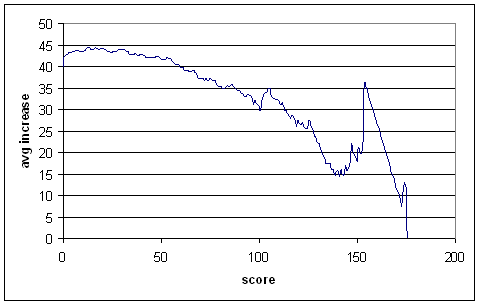
This is similar to the Test graph — batsmen clearly get their eye in after scoring some runs — but the downward trend starts much earlier, as is expected. After about 60 runs, the average increases are less than the overall average for this dataset (almost exactly 40). So not-outs tend to deflate averages when the score is below 60, but inflates them afterwards.
And now for the middle order:
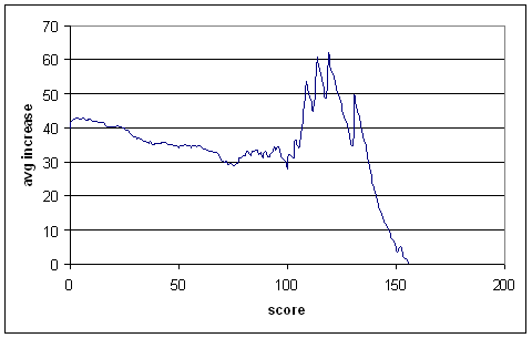
I wouldn't pay much attention to the curve out past 100, since there's not much data there. It won't make too much difference, since there aren't that many unbeaten centuries in the middle order.
The curve is quite different from that of the top order, in roughly the way we would expect. Not-outs have a deflating effect on averages only up to 25 runs or so, and after that they inflate averages.
Now, I haven't done a thorough analysis on all batsmen, since I don't have that data handy. I've just done some selected cases. Some caveats: Some of the batsmen played earlier than ten years ago, and perhaps the average increase curves was different then. Also, I've applied either top order or middle order adjustments to each batsman, and not both. This won't have too much of an effect, but to do it properly you'd want to split the innings into top-order and middle-order and do them separately. If a batsman's highest score was a not-out, I added the average increase to it. (For Tests, I added the batsman's regular average, but doing so in ODI's is much less accurate.)
In the table below there are four averages presented: the regular average, one adjusted based purely on the batsman's own scores, one based purely on the relevant graph above (shifted up or down to match the batsman's regular average), and one mixture of the two, giving more weight to the graph when the batsman doesn't have many scores greater than or equal to the not-out being projected. I've called these reg, ind, gph, mix. The latter one is the one I'd go with. There's two openers, and the rest from the middle order.
Bevan's average has, contrary to my expectations, been pulled back quite a bit, down below 49. Nevertheless, it's still a lot higher than most Bevan sceptics would have it. I wouldn't want to draw too many general conclusions from what was a deliberately biased set of batsmen (all with fairly high not-out proportions), but it looks like ODI averages can be and sometimes are inflated by not-outs much more than Test averages.
(Usually I'd rather watch paint dry than copy-paste Statsguru data for an hour, but it's not so bad you're listening to the Champions League football on the radio.)
There's one very important difference for this exercise between ODI's and Tests. In Tests, pretty much all the top batsmen can expect to bat out their innings most of the time. In ODI's, the top order can usually do this, but the middle order often have to slog at the end. So whereas an opener can get a start of 50 and carry on to a century, the number six who gets to 50 will often get out soon afterwards.
So I split the analysis into two parts: one for the top order (1-3), and one for the middle order (4-7). Perhaps 1-4 and 5-7 would have been better, but I can hardly be bothered re-gathering the data.
I only considered batsmen with an average of 35 or more, and only considered innings in the last ten years, since there's been a big explosion in ODI run habits recently.
First up, projected increases for the top order:

This is similar to the Test graph — batsmen clearly get their eye in after scoring some runs — but the downward trend starts much earlier, as is expected. After about 60 runs, the average increases are less than the overall average for this dataset (almost exactly 40). So not-outs tend to deflate averages when the score is below 60, but inflates them afterwards.
And now for the middle order:

I wouldn't pay much attention to the curve out past 100, since there's not much data there. It won't make too much difference, since there aren't that many unbeaten centuries in the middle order.
The curve is quite different from that of the top order, in roughly the way we would expect. Not-outs have a deflating effect on averages only up to 25 runs or so, and after that they inflate averages.
Now, I haven't done a thorough analysis on all batsmen, since I don't have that data handy. I've just done some selected cases. Some caveats: Some of the batsmen played earlier than ten years ago, and perhaps the average increase curves was different then. Also, I've applied either top order or middle order adjustments to each batsman, and not both. This won't have too much of an effect, but to do it properly you'd want to split the innings into top-order and middle-order and do them separately. If a batsman's highest score was a not-out, I added the average increase to it. (For Tests, I added the batsman's regular average, but doing so in ODI's is much less accurate.)
In the table below there are four averages presented: the regular average, one adjusted based purely on the batsman's own scores, one based purely on the relevant graph above (shifted up or down to match the batsman's regular average), and one mixture of the two, giving more weight to the graph when the batsman doesn't have many scores greater than or equal to the not-out being projected. I've called these reg, ind, gph, mix. The latter one is the one I'd go with. There's two openers, and the rest from the middle order.
player        inns  no  reg   ind   gph   mix
SR Tendulkar  407   38  44,3  43,4  43,9  43,5
SC Ganguly    300   23  41,0  40,6  40,6  40,6
---
MG Bevan      196   67  53,6  48,1  52,4  48,8
L Klusener    137   50  41,1  41,7  40,1  41,4
MEK Hussey    64    26  55,6  55,0  54,4  54,9
A Symonds     154   32  39,7  40,1  39,0  39,9
DR Martyn     182   51  40,8  42,1  40,0  41,6
RP Arnold     155   43  35,3  33,5  34,6  33,8
Bevan's average has, contrary to my expectations, been pulled back quite a bit, down below 49. Nevertheless, it's still a lot higher than most Bevan sceptics would have it. I wouldn't want to draw too many general conclusions from what was a deliberately biased set of batsmen (all with fairly high not-out proportions), but it looks like ODI averages can be and sometimes are inflated by not-outs much more than Test averages.
Sunday, April 06, 2008
Largest deficits to win
Something a little less full-on today, back to first-class trivia. The largest first innings deficit leading to a win is 402 runs, in this match. But it was a contrived result: Central Districts made 464, Northern Districts replied with 2dec/62, Central 0dec/26, Northern 8/429 won by two wickets. Ignoring matches where the team batting second declared behind, and also ignoring the forfeited Test, the top five deficits to win are (up to the end of the 2007 English season):
384: Barbados 175 & 7dec/726 def. Trinidad 559 & 217, 1926/7
291: Australia 256 & 471 def. Sri Lanka 8dec/547 & 164, 1992/3
287: Manicaland 9dec/513 & 146 lost to Mashonaland 226 & 506 (f/o), 2001/2
279: Western Province 460 & 3dec/219 lost to South African Universities 181 & 7/500, 1978/9
277: Nottinghamshire 4dec/431 & 0dec/94 lost to Lancashire 154 & 4/372, 1961
I can only find two instances of a batsman being out stumped X bowled Y in the first innings, and stumped Y bowled X in the second. They are Frederick Thackeray in this match (st: Cobbett b: Bayley in the first innings, st: Bayley b: Cobbett in the second) in 1839, and Ron Oxenham in this match (st: Strudwick b: Freemand in the first innings, st: Freemand b: Strudwick in the second) in 1924/5.
Saturday, April 05, 2008
Slumps - Is there a problem or is he just unlucky?
I've had a bit of a think about "form slumps", and how we might go about seeing if they're just due to chance (sometimes a batsmen will be dismissed for a string of low scores) or due to some genuine problem (a technique flaw, or a weakness found by opposition bowlers). This post becomes more technical than usual later on, so feel free to fall asleep after the first table. This may not be the best or fastest way of going about this problem, but it's they way I did go about it — sort of like stream of consciousness statistics. The important thing is that it works, and it doesn't require anything more than Excel.
The first thing we need to know is the distribution of individual innings scores. Actually we don't need that — we just need to know what the standard deviation is, relative to the mean. So, for each batsman with 50 Test innings or more and an average of at least 35, I calculated the coefficient of variation (the standard deviation divided by the mean). This is a measure of the consistency of a batsman. My own opinion is that consistency is over-rated — a batsman who goes 0, 100, 0, 100, etc. is just as useful as a batsman who goes 50, 50, 50, etc. But it is still interesting to see which batsmen are more consistent than others, so here's the top and bottom of the table. A higher co-efficient of variation means less consistency.
(Technical note: for not-outs, I just added the batsman's average and considered it a regular innings. Not the best thing to do, but it's close enough, and we'll be doing far worse later on.)
There is only a very slight trend (R-squared = 0,022) showing higher averages associated with lower co-efficients of variation.
The average co-efficient of variation is about 1,05. From now on we'll ignore individual differences between batsmen and just assume that the scores of each batsmen can be treated as random variables, coming from a distribution with mean µ (i.e., his average) and standard deviation 1,05µ.
No, we're interested in slumps. So instead of considering individual innings, we'll be considering groups of innings. We don't know what the distribution of individual innings is exactly, but the distribution of groups of innings will be approximately normal, by the central limit theorem. In particular, the mean of a group of n innings will be approximately normally distributed with mean µ (the same as the career average) and standard deviation 1,05µ/sqrt(n).
Note that while I said that µ was the career average, in order for things to work out properly, we'll actually use the career average apart from the slump in question.
So, to define how bad a slump of n innings is, we'll calculate a z-score. Let µc be the career average (excluding the slump) and µs be the average during the slump. Then define z = (µs - µc) * sqrt(n) / (1,05 * µc).
For example, suppose a batsman was averaging 45. Then he had a slump where for 25 innings he averaged 30. The z-score here would be (30 - 45) * sqrt(25) / (1,05 * 45) = -1,59. I'll call this a z = -1,59 slump.
How rare is this sort of slump? We can look up the answer in either a cumulative normal distribution table or use Excel (or something fancier). In Excel, the relevant function in French is LOI.NORMALE.STANDARD(z). For that small minority of you who use computers set to English, I think the function is called NORMSDIST.
Anyway, plug in -1,59 and you get 0,056. So, that tells us that the probability that he'd have a slump that bad (or worse) right now is about 5,6%. Does the theory match reality? For each batsman, I considered blocks of 26 innings (26 and not 25 for reasons that were important to me when I was testing this but don't make any difference now) that didn't overlap. It's important that they don't overlap, because otherwise the probabilities will be dependent. Add up the number of slumps worse than a particular z, divide by the total number of blocks sampled, and you get a probability. Here are the results, for varying z's, with the observed probability and that derived from the normal distribution.
That's not too bad. The observed probabilities are low in the tail, but we'd be talking about really really bad slumps out there, so that's not too important. For the z=-1,59 slump in the example above (something reasonably typical), we see that it matches pretty closely. From now on, we'll just use the normal distribution instead of the empirically derived probabilities.
So the theory works well enough. But we can't stop here. The probability of a z = -1,59 slump right now is about 5,6%. But that's not what we're interested in. We'd like to know the probability that at some point during a batsman's career, he'll have a z = -1,59 slump. This is a very different thing entirely! The probability of a batsman making a duck is about 6,5%, but you wouldn't call it a slump if he's just made a duck, because ducks are just going to happen sometimes.
So how do we find the probability, given a career of M innings, that there'll be a z = -1,59 slump in there somewhere. To answer this (perhaps not in the best way), let's review some basic probability.
Imagine you roll a die five times. What's the probability that you get at least one 6? You can't say: "The probability of a 6 on any roll is 1/6, so the probability of getting a 6 after five rolls is 5/6." That would be the expectation of how many 6's you get. What you need to do is find the probability that you won't get a 6 on each roll — 5/6 — raise that to the fifth power (probability that you won't get a 6 in five rolls), then subtract it from 1. The answer is about 0,598.
So, suppose a career is 80 innings long. A slump of 20 innings could start at innings 1, innings 2, ..., innings 61. So, do we take our probability of 0,056 from above, subtract from 1, raise to the power of 61, subtract from 1? No! Because when you take blocks of innings that overlap with each other, you're looking at dependent events. Two rolls of the die won't affect each other. But the average of innings 2 to 21 will be highly dependent on the average from innings 1 to 20 — after all, 19 of the innings are in both blocks.
So we can't just raise that probability to the 61st power. So what can we do? I don't know what the best way is, but I decided to numerically work out what power you should raise (1 - 0,056) to.
So, summary of the procedure so far:
1. Find z.
2. Get associated probability pnow = LOI.NORMALE.STANDARD(z).
3. Raise (1 - pnow) to some power x, to be determined numerically.
4. Find 1 - (1 - pnow)x. This is the probability of having a z-slump at some point during the career.
But, when I was working through this, I accidentally cut out the last step. Happily, I get much better fits this way (I did try doing following the above procedure afterwards), but the exponent that you get doesn't have the same nice interpretation as the one above.
So, actual procedure:
1. Find z.
2. Get associated probability pnow = LOI.NORMALE.STANDARD(z).
3. Raise (1 - pnow) to some power x, to be determined numerically. This is the probability of having a z-slump at some point during the career.
So, time to work out x. The first thing we'll see is that the ratio of the career length to slump length is important — for a given ratio, it doesn't matter so much what the length of the slump is. So x will be the same for a 40-innings slump in a 120-innings career as for a 20-innings slump in a 60-innings career.
If N is the length of the career and n the length of the slump, then the ratio I actually worked with (just by 'historical accident) was (N + 1 - n) / N.
Let's plot x against z for 20-innings slumps in 79-innings careers:

It's a nice exponential fit. Repeating the procedure for other block sizes (always with length ratio of 3), you get the following table (fit parameters here are the A and k in x = Ae-kz):
The co-efficients can be sensitive to how much of the tail you let in, but basically they don't change too much. You might be thinking, "Hey! There's almost a factor of 2 difference there!" We'll ignore that and see what happens later.
Now we'll hold the slump length constant (at 26) and vary the ratio. Resulting graph of the fit parameter A:

It's another exponential decay.
Resulting graph for fit parameter k:

It's linear.
You can see that I've gone up to a ratio of 5. Much past that and I start running into lack of data problems, though I could probably have kept going with more thought and patience.
So, now we have all we need. Full procedure for finding the probability that a batsmen will have a particular z-slump of length n during his career of length N:
1. Calculate his average over the slump µs, and his career average excluding the slump µc.
2. Calculate z = (µs - µc) * sqrt(n) / (1,05 * µc).
3. Find pnow = LOI.NORMALE.STANDARD(z).
4. Find q = (N + 1 - n) / n.
5. Find A = 0,25 * e-1,4*q.
6. Find k = -(0,62 * q + 2,96).
7. Find x = A * ek * z.
8. Find p = (1 - pnow)x.
So does it work? Let's have a look at observed probabilites and the p as calculated above for a 20-innings slump in a 79-innings career:
Wrong way out in the tail, but pretty good for z greater than -2 or so.
What about a 15-innings slump in a 134-innings career? That's outside the regions we used to derive the fit parameters.
Pretty good.
Now, if I were a selector who never actually watched the players and only looked at the scores they made, how would I used this in practice? Well, if a particular batsmen was in a slump, I'd want to know how likely it is that that sort of slump would happen in a career as long as his. If it's more than 50%, then I'd let him keep going. If it's less than 50%, I'd drop him.
A practical example: Andrew Strauss. Before his much-publicised recent slump, he averaged 46,39. During the slump, up to the second Test against New Zealand, he averaged 28,10. The slump lasted 29 innings; his career up to then had lasted 83 innings.
So:
1. µs = 28,10; µc = 46,39.
2. z = (28,10 - 46,39) * sqrt(29) / (1,05 * 46,39) = -2,02.
3. pnow = LOI.NORMALE.STANDARD(-2,02) = 0,0217.
4. q = (83 + 1 - 29) / 29 = 1,90.
5. A = 0,25 * e-1,4 * 1,90 = 0,0176.
6. k = -(0,62 * 1,90 + 2,96) * (-2,02) = 8,359.
7. x = A * ek = 75,1.
8. p = (1 - 0,0217)75,1 = 0,192.
So slumps as bad as Strauss's should only happen to about one player in five, in a career as long as his. So based on numbers alone, I would have dropped him. Of course, he hit 177 in his next Test.
Now I think that this has been a useful exercise, but I'm not sure how much use it has in practice. You don't pick cricket teams based purely on statistics — you have to watch the players as well. If (say) a batsman is regularly getting out LBW early in his innings, you don't want to let it keep happening until p becomes 0,5 before dropping him. You want to get in early, and either drop him or work on his technique.
The first thing we need to know is the distribution of individual innings scores. Actually we don't need that — we just need to know what the standard deviation is, relative to the mean. So, for each batsman with 50 Test innings or more and an average of at least 35, I calculated the coefficient of variation (the standard deviation divided by the mean). This is a measure of the consistency of a batsman. My own opinion is that consistency is over-rated — a batsman who goes 0, 100, 0, 100, etc. is just as useful as a batsman who goes 50, 50, 50, etc. But it is still interesting to see which batsmen are more consistent than others, so here's the top and bottom of the table. A higher co-efficient of variation means less consistency.
(Technical note: for not-outs, I just added the batsman's average and considered it a regular innings. Not the best thing to do, but it's close enough, and we'll be doing far worse later on.)
name            inns  avg     sd      cv
MH Richardson   65    44,77   35,72   0,80
H Sutcliffe     84    60,73   48,52   0,80
JB Hobbs        102   56,95   48,53   0,85
AN Cook         51    43,47   37,83   0,87
PE Richardson   56    37,47   32,91   0,88
A Ranatunga     155   35,70   31,40   0,88
IR Redpath      120   43,46   38,62   0,89
NC O'Neill      69    45,56   40,72   0,89
KF Barrington   131   58,67   52,50   0,90
JB Stollmeyer   56    42,33   37,98   0,90
---
Ijaz Ahmed      92    37,67   46,07   1,22
DN Sardesai     55    39,24   48,54   1,24
V Sehwag        90    53,76   66,76   1,24
VT Trumper      89    39,05   48,57   1,24
Zaheer Abbas    124   44,80   56,86   1,27
Hanif Mohammad  97    43,99   55,81   1,27
DL Amiss        88    46,31   60,59   1,31
JA Rudolph      63    36,21   47,99   1,33
W Jaffer        54    35,68   48,09   1,35
MS Atapattu     156   39,02   52,81   1,35
There is only a very slight trend (R-squared = 0,022) showing higher averages associated with lower co-efficients of variation.
The average co-efficient of variation is about 1,05. From now on we'll ignore individual differences between batsmen and just assume that the scores of each batsmen can be treated as random variables, coming from a distribution with mean µ (i.e., his average) and standard deviation 1,05µ.
No, we're interested in slumps. So instead of considering individual innings, we'll be considering groups of innings. We don't know what the distribution of individual innings is exactly, but the distribution of groups of innings will be approximately normal, by the central limit theorem. In particular, the mean of a group of n innings will be approximately normally distributed with mean µ (the same as the career average) and standard deviation 1,05µ/sqrt(n).
Note that while I said that µ was the career average, in order for things to work out properly, we'll actually use the career average apart from the slump in question.
So, to define how bad a slump of n innings is, we'll calculate a z-score. Let µc be the career average (excluding the slump) and µs be the average during the slump. Then define z = (µs - µc) * sqrt(n) / (1,05 * µc).
For example, suppose a batsman was averaging 45. Then he had a slump where for 25 innings he averaged 30. The z-score here would be (30 - 45) * sqrt(25) / (1,05 * 45) = -1,59. I'll call this a z = -1,59 slump.
How rare is this sort of slump? We can look up the answer in either a cumulative normal distribution table or use Excel (or something fancier). In Excel, the relevant function in French is LOI.NORMALE.STANDARD(z). For that small minority of you who use computers set to English, I think the function is called NORMSDIST.
Anyway, plug in -1,59 and you get 0,056. So, that tells us that the probability that he'd have a slump that bad (or worse) right now is about 5,6%. Does the theory match reality? For each batsman, I considered blocks of 26 innings (26 and not 25 for reasons that were important to me when I was testing this but don't make any difference now) that didn't overlap. It's important that they don't overlap, because otherwise the probabilities will be dependent. Add up the number of slumps worse than a particular z, divide by the total number of blocks sampled, and you get a probability. Here are the results, for varying z's, with the observed probability and that derived from the normal distribution.
z     obs     loi normale
-3,0  0       0,001
-2,9  0       0,002
-2,8  0,000   0,003
-2,7  0,001   0,003
-2,6  0,001   0,005
-2,5  0,002   0,006
-2,4  0,004   0,008
-2,3  0,006   0,011
-2,2  0,008   0,014
-2,1  0,012   0,018
-2,0  0,018   0,023
-1,9  0,023   0,029
-1,8  0,032   0,036
-1,7  0,041   0,045
-1,6  0,053   0,055
-1,5  0,066   0,067
-1,4  0,080   0,081
-1,3  0,095   0,097
-1,2  0,111   0,115
-1,1  0,134   0,136
That's not too bad. The observed probabilities are low in the tail, but we'd be talking about really really bad slumps out there, so that's not too important. For the z=-1,59 slump in the example above (something reasonably typical), we see that it matches pretty closely. From now on, we'll just use the normal distribution instead of the empirically derived probabilities.
So the theory works well enough. But we can't stop here. The probability of a z = -1,59 slump right now is about 5,6%. But that's not what we're interested in. We'd like to know the probability that at some point during a batsman's career, he'll have a z = -1,59 slump. This is a very different thing entirely! The probability of a batsman making a duck is about 6,5%, but you wouldn't call it a slump if he's just made a duck, because ducks are just going to happen sometimes.
So how do we find the probability, given a career of M innings, that there'll be a z = -1,59 slump in there somewhere. To answer this (perhaps not in the best way), let's review some basic probability.
Imagine you roll a die five times. What's the probability that you get at least one 6? You can't say: "The probability of a 6 on any roll is 1/6, so the probability of getting a 6 after five rolls is 5/6." That would be the expectation of how many 6's you get. What you need to do is find the probability that you won't get a 6 on each roll — 5/6 — raise that to the fifth power (probability that you won't get a 6 in five rolls), then subtract it from 1. The answer is about 0,598.
So, suppose a career is 80 innings long. A slump of 20 innings could start at innings 1, innings 2, ..., innings 61. So, do we take our probability of 0,056 from above, subtract from 1, raise to the power of 61, subtract from 1? No! Because when you take blocks of innings that overlap with each other, you're looking at dependent events. Two rolls of the die won't affect each other. But the average of innings 2 to 21 will be highly dependent on the average from innings 1 to 20 — after all, 19 of the innings are in both blocks.
So we can't just raise that probability to the 61st power. So what can we do? I don't know what the best way is, but I decided to numerically work out what power you should raise (1 - 0,056) to.
So, summary of the procedure so far:
1. Find z.
2. Get associated probability pnow = LOI.NORMALE.STANDARD(z).
3. Raise (1 - pnow) to some power x, to be determined numerically.
4. Find 1 - (1 - pnow)x. This is the probability of having a z-slump at some point during the career.
But, when I was working through this, I accidentally cut out the last step. Happily, I get much better fits this way (I did try doing following the above procedure afterwards), but the exponent that you get doesn't have the same nice interpretation as the one above.
So, actual procedure:
1. Find z.
2. Get associated probability pnow = LOI.NORMALE.STANDARD(z).
3. Raise (1 - pnow) to some power x, to be determined numerically. This is the probability of having a z-slump at some point during the career.
So, time to work out x. The first thing we'll see is that the ratio of the career length to slump length is important — for a given ratio, it doesn't matter so much what the length of the slump is. So x will be the same for a 40-innings slump in a 120-innings career as for a 20-innings slump in a 60-innings career.
If N is the length of the career and n the length of the slump, then the ratio I actually worked with (just by 'historical accident) was (N + 1 - n) / N.
Let's plot x against z for 20-innings slumps in 79-innings careers:

It's a nice exponential fit. Repeating the procedure for other block sizes (always with length ratio of 3), you get the following table (fit parameters here are the A and k in x = Ae-kz):
slump length  A       k
20            0,0026  -4,97
26            0,0018  -5,05
30            0,0018  -5,08
40            0,0033  -4,90
The co-efficients can be sensitive to how much of the tail you let in, but basically they don't change too much. You might be thinking, "Hey! There's almost a factor of 2 difference there!" We'll ignore that and see what happens later.
Now we'll hold the slump length constant (at 26) and vary the ratio. Resulting graph of the fit parameter A:

It's another exponential decay.
Resulting graph for fit parameter k:

It's linear.
You can see that I've gone up to a ratio of 5. Much past that and I start running into lack of data problems, though I could probably have kept going with more thought and patience.
So, now we have all we need. Full procedure for finding the probability that a batsmen will have a particular z-slump of length n during his career of length N:
1. Calculate his average over the slump µs, and his career average excluding the slump µc.
2. Calculate z = (µs - µc) * sqrt(n) / (1,05 * µc).
3. Find pnow = LOI.NORMALE.STANDARD(z).
4. Find q = (N + 1 - n) / n.
5. Find A = 0,25 * e-1,4*q.
6. Find k = -(0,62 * q + 2,96).
7. Find x = A * ek * z.
8. Find p = (1 - pnow)x.
So does it work? Let's have a look at observed probabilites and the p as calculated above for a 20-innings slump in a 79-innings career:
z     obs     p
-3,0  0       0,000
-2,9  0       0,000
-2,8  0       0,001
-2,7  0,008   0,003
-2,6  0,008   0,008
-2,5  0,039   0,018
-2,4  0,086   0,038
-2,3  0,117   0,071
-2,2  0,148   0,120
-2,1  0,211   0,186
-2,0  0,289   0,265
-1,9  0,336   0,354
-1,8  0,398   0,447
-1,7  0,531   0,538
-1,6  0,602   0,623
-1,5  0,695   0,699
-1,4  0,734   0,764
-1,3  0,813   0,818
-1,2  0,859   0,861
-1,1  0,969   0,896
Wrong way out in the tail, but pretty good for z greater than -2 or so.
What about a 15-innings slump in a 134-innings career? That's outside the regions we used to derive the fit parameters.
-2,1  0,390   0,353
-2,0  0,542   0,548
-1,9  0,678   0,708
-1,8  0,780   0,821
-1,7  0,814   0,895
-1,6  0,848   0,940
-1,5  0,864   0,966
-1,4  0,966   0,981
-1,3  0,983   0,990
-1,2  0,983   0,994
Pretty good.
Now, if I were a selector who never actually watched the players and only looked at the scores they made, how would I used this in practice? Well, if a particular batsmen was in a slump, I'd want to know how likely it is that that sort of slump would happen in a career as long as his. If it's more than 50%, then I'd let him keep going. If it's less than 50%, I'd drop him.
A practical example: Andrew Strauss. Before his much-publicised recent slump, he averaged 46,39. During the slump, up to the second Test against New Zealand, he averaged 28,10. The slump lasted 29 innings; his career up to then had lasted 83 innings.
So:
1. µs = 28,10; µc = 46,39.
2. z = (28,10 - 46,39) * sqrt(29) / (1,05 * 46,39) = -2,02.
3. pnow = LOI.NORMALE.STANDARD(-2,02) = 0,0217.
4. q = (83 + 1 - 29) / 29 = 1,90.
5. A = 0,25 * e-1,4 * 1,90 = 0,0176.
6. k = -(0,62 * 1,90 + 2,96) * (-2,02) = 8,359.
7. x = A * ek = 75,1.
8. p = (1 - 0,0217)75,1 = 0,192.
So slumps as bad as Strauss's should only happen to about one player in five, in a career as long as his. So based on numbers alone, I would have dropped him. Of course, he hit 177 in his next Test.
Now I think that this has been a useful exercise, but I'm not sure how much use it has in practice. You don't pick cricket teams based purely on statistics — you have to watch the players as well. If (say) a batsman is regularly getting out LBW early in his innings, you don't want to let it keep happening until p becomes 0,5 before dropping him. You want to get in early, and either drop him or work on his technique.
Subscribe to Comments [Atom]