Friday, April 11, 2008
Getting your eye in
(Update: See these two followup posts.)
An anonymous commenter pointed me to arXiv:0801.4408v1, a paper by Brendon Brewer called "Getting Your Eye In: A Bayesian Analysis of Early Dismissals in Cricket".
Before starting the discussion, I'll define the hazard function. These seem to be used all over the place in the (pretty small) academic literature on cricket scores. The hazard function, written H(x), is defined as the probability that the batsman will be dismissed at score x.
Simple enough. But Brewer points out a very neat interpretation of it (he may not be the first to do so, but it's the first time I've seen it). If the hazard function is constant (i.e., always equal probability of getting out), you get a geometric distribution of scores (or, in the continuous limit, the exponential distribution that I mention every couple of weeks). In particular, a hazard value H is related to a batting average µ by µ = 1/H - 1.
So (here's the important bit), given a particular value of H for some batsman (say H(0) = 0,06 — the probability of making a duck), we can say that, on zero, he bats like someone with an average of 1/0,06 - 1 = 15,67. If you're not convinced that this is useful, you should be by the end of this post.
Technical details follow. Feel free to skip to the tables below.
The methods used in the paper are too technical for me to be bothered understanding them all, but here is a brief summary:
- Assume that the hazard function is of a particular type depending on various parameters.
- Estimate what those parameters are.
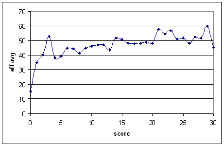
I think that the main problem with the assumptions is that they don't take into account how important getting off the mark is. It's assumed that it's a pretty smooth transition from zero to some higher score. But, if you work out the hazard directly (I took all batsmen who average over 40 in Tests), you get this:

There's an almost 20-run jump in effective average from a score of zero to a score of one. (Also, it curve doesn't level off for a long time.)
So, I instead took assumed that the average associated with the hazard goes like:
µ = a + k*(b - a)*xp.
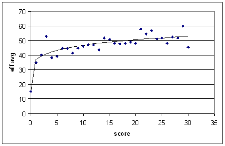
I originally intended for all of those parameters to have nice interpretations, but the actual results made a mockery of that idea. Anyway, if you fit the graph above up to x = 30, you get the following (fit parameters: a = 15,2; b = 49,4; k = 0,63; p = 0,17):

Technical notes: I did the fits using gretl's non-linear least squares abilities. You do the fits with the hazard function and then convert to an average, since sometimes the hazard function gets close to or equal to zero. If you convert to an average before fitting, you get some data points heading off to infinity and nothing works. I used scores from 0 to 49. The way the equation's set up, the parameter 'a' basically picks out the empirical hazard at zero. I think that this is reasonable, since getting off the mark is so important. But it's debatable.
Unfortunately, I don't know how to automate everything, so I have to do one batsman at a time. Maybe next time I'm listening to football on the radio I'll go through and process a bunch of batsmen.
Now, the parameter 'a' does have a nice interpretation: it's the effective batting average at zero. The parameter 'p' tells you how flat the curve is (near zero: very flat). While I give the values of the parameters for each player, the more important thing is the effective average µ at various scores. I've given µ(0) (which is just 'a'), µ(1) (effective average at 1), µ(10), and µ(30). There's a bit of round-off error (I went gretl -> pen and paper -> Excel), but it's nothing serious. I've also given the regular average in the last column.
To start with, here's the very atypical example of Don Bradman:
Don't let Bradman get off the mark! On zero he batted like someone who averaged 10, but on one he was almost as good as Mike Hussey. Very soon he batted like the best batsmen ever. Bradman's apparent woefulness before he got off the mark seems pretty typical. Let's have a look at some others.
Interestingly, the two best batsmen on nought are Langer and Kirsten — both openers. Unfortunately, this is a (very) limited dataset, so we'll put this aside for further study.
In Brewer's own small dataset, he saw that the two all-rounders had little change from "before eye in" to "eye in". Part of that I think is due to the wrong shape of the hazard function, but all-rounders doing well on nought does seem to be a real effect (again, pending a more thorough study):
In terms of flatness of the effective average (once off the mark), I think the most important factor is the regular average. Sorta-all-right batsmen who average 30 will typically get lots of starts but not go on with them. Two examples (again it'd be nice to have more, but I didn't cherrypick — they were the only two I looked at):
So players like Ramprakash and Mahanama have got their eye in once they're off the mark, but that's as far as it goes. Better batsmen continue to improve, but these ones don't, for whatever reasons.
That's all I have for now. Feel free to make requests, and to make it interesting, say what you think the results will be for each batsman (e.g., terrible on zero, good on zero, etc.).
And I hope you're all convinced that the effective average is a wonderful number for this exercise.
An anonymous commenter pointed me to arXiv:0801.4408v1, a paper by Brendon Brewer called "Getting Your Eye In: A Bayesian Analysis of Early Dismissals in Cricket".
Before starting the discussion, I'll define the hazard function. These seem to be used all over the place in the (pretty small) academic literature on cricket scores. The hazard function, written H(x), is defined as the probability that the batsman will be dismissed at score x.
Simple enough. But Brewer points out a very neat interpretation of it (he may not be the first to do so, but it's the first time I've seen it). If the hazard function is constant (i.e., always equal probability of getting out), you get a geometric distribution of scores (or, in the continuous limit, the exponential distribution that I mention every couple of weeks). In particular, a hazard value H is related to a batting average µ by µ = 1/H - 1.
So (here's the important bit), given a particular value of H for some batsman (say H(0) = 0,06 — the probability of making a duck), we can say that, on zero, he bats like someone with an average of 1/0,06 - 1 = 15,67. If you're not convinced that this is useful, you should be by the end of this post.
Technical details follow. Feel free to skip to the tables below.
The methods used in the paper are too technical for me to be bothered understanding them all, but here is a brief summary:
- Assume that the hazard function is of a particular type depending on various parameters.
- Estimate what those parameters are.
I think that the main problem with the assumptions is that they don't take into account how important getting off the mark is. It's assumed that it's a pretty smooth transition from zero to some higher score. But, if you work out the hazard directly (I took all batsmen who average over 40 in Tests), you get this:

There's an almost 20-run jump in effective average from a score of zero to a score of one. (Also, it curve doesn't level off for a long time.)
So, I instead took assumed that the average associated with the hazard goes like:
µ = a + k*(b - a)*xp.
I originally intended for all of those parameters to have nice interpretations, but the actual results made a mockery of that idea. Anyway, if you fit the graph above up to x = 30, you get the following (fit parameters: a = 15,2; b = 49,4; k = 0,63; p = 0,17):

Technical notes: I did the fits using gretl's non-linear least squares abilities. You do the fits with the hazard function and then convert to an average, since sometimes the hazard function gets close to or equal to zero. If you convert to an average before fitting, you get some data points heading off to infinity and nothing works. I used scores from 0 to 49. The way the equation's set up, the parameter 'a' basically picks out the empirical hazard at zero. I think that this is reasonable, since getting off the mark is so important. But it's debatable.
Unfortunately, I don't know how to automate everything, so I have to do one batsman at a time. Maybe next time I'm listening to football on the radio I'll go through and process a bunch of batsmen.
Now, the parameter 'a' does have a nice interpretation: it's the effective batting average at zero. The parameter 'p' tells you how flat the curve is (near zero: very flat). While I give the values of the parameters for each player, the more important thing is the effective average µ at various scores. I've given µ(0) (which is just 'a'), µ(1) (effective average at 1), µ(10), and µ(30). There's a bit of round-off error (I went gretl -> pen and paper -> Excel), but it's nothing serious. I've also given the regular average in the last column.
To start with, here's the very atypical example of Don Bradman:
player        b     k     p     µ(0)  µ(1)  µ(10) µ(30) avg
DG Bradman    71,3  0,96  0,13  10,4  68,9  89,3  101,4 99,9
Don't let Bradman get off the mark! On zero he batted like someone who averaged 10, but on one he was almost as good as Mike Hussey. Very soon he batted like the best batsmen ever. Bradman's apparent woefulness before he got off the mark seems pretty typical. Let's have a look at some others.
player        b     k     p     µ(0)  µ(1)  µ(10) µ(30) avg
SR Waugh      50,3  0,56  0,22  10,7  32,9  47,5  57,6  51,1
N Hussain     38,2  0,53  0,29  11,3  25,6  39,1  49,5  37,2
JL Langer     56,3  0,63  0,026 16,9  41,7  43,3  44,0  45,7
G Kirsten     61,6  0,24  0,41  12,4  24,2  42,8  60,0  45,3
BC Lara       199,0 0,11  0,25  12,5  33,0  49,0  60,5  53,2
ME Waugh      70,6  0,39  0,18  10,0  33,6  45,8  53,6  41,8
Interestingly, the two best batsmen on nought are Langer and Kirsten — both openers. Unfortunately, this is a (very) limited dataset, so we'll put this aside for further study.
In Brewer's own small dataset, he saw that the two all-rounders had little change from "before eye in" to "eye in". Part of that I think is due to the wrong shape of the hazard function, but all-rounders doing well on nought does seem to be a real effect (again, pending a more thorough study):
player        b     k     p     µ(0)  µ(1)  µ(10) µ(30) avg
SM Pollock    44,2  0,53  0,026 16,2  31,0  32,0  32,4  32,3
CL Cairns     43,2  0,39  0,28  14,2  25,5  35,8  43,5  33,5
GStA Sobers   68,2  0,75  1E-08 12,4  54,3  54,3  54,3  57,8
Imran Khan    48,7  0,55  0,052 14,9  33,5  35,9  37,1  37,7
GA Faulkner   31,7  0,13  1,02  26,4  27,1  33,6  48,5  40,8
JH Kallis     68,2  0,56  0,13  18,6  46,4  56,1  61,8  57,1
KR Miller     50,8  0,48  0,086 16,6  33,0  36,6  38,6  37,0
In terms of flatness of the effective average (once off the mark), I think the most important factor is the regular average. Sorta-all-right batsmen who average 30 will typically get lots of starts but not go on with them. Two examples (again it'd be nice to have more, but I didn't cherrypick — they were the only two I looked at):
player        b     k     p     µ(0)  µ(1)  µ(10) µ(30) avg
MR Ramprakash 52,3  0,49  1E-08 6,7   29,1  29,1  29,1  27,3
RS Mahanama   51,1  0,40  0,037 11,7  27,5  28,9  29,6  29,3
So players like Ramprakash and Mahanama have got their eye in once they're off the mark, but that's as far as it goes. Better batsmen continue to improve, but these ones don't, for whatever reasons.
That's all I have for now. Feel free to make requests, and to make it interesting, say what you think the results will be for each batsman (e.g., terrible on zero, good on zero, etc.).
And I hope you're all convinced that the effective average is a wonderful number for this exercise.
Comments:
<< Home
I think captains do tend to attack new batsmen though - there's almost always an extra couple of slips in for the new batsmen. And more attacking fields make it easier for the batsman to score runs, so it's a trade-off.
If you are interested in automation, perhaps you might try investing in MATLAB (http://www.mathworks.com). It's powerful and easy to use (for me anyway) and it can import excel files so no worries there.
I'd like to see how your hazard function deals with the 'poor starters'. People like S Waugh and Ponting (I am Australian, if you can't tell). And maybe you could compare them to the 'blazers', ie. Gilchrist, V Richards, Sehwag &etc. My theory is they will both jump significantly after the first run (like Sobers does).
I'd like to see how your hazard function deals with the 'poor starters'. People like S Waugh and Ponting (I am Australian, if you can't tell). And maybe you could compare them to the 'blazers', ie. Gilchrist, V Richards, Sehwag &etc. My theory is they will both jump significantly after the first run (like Sobers does).
Thanks Michael. I've worked out how to write scripts for gretl now, so I've now got it automated.
Interestingly, Ponting's not a bad starter - µ(0) = 23. In general, you're right that poor starters have bigger jumps once off the mark. Taking all batsmen (excluding a couple with poorly-behaved hazard functions) who average 35 or more, a regression on µ(1) - µ(0) against µ(0) gives
µ(1) - µ(0) = -0,73*µ(0) + 31,4. R-squared of 0,38. So those who start poorly jump up more once off the mark. Now there's a bit of a selection effect here - they all have pretty good (or better) averages, so they have to start getting better at some point. But it seems that much of that improvement comes once off the mark.
Now for some fast scorers. (I don't have strike rate data, so I'm just picking players here.)
player: µ(0); µ(1); µ(10); µ(30)
Sehwag: 9,0; 44,2; 44,2; 44,2
Gilchrist: 8,6; 26,4; 45,5; 60,8
Pietersen: 22,2; 44,7; 44,7; 44,7
Jayasuriya: 11,5; 38,4; 39,4; 39,9
McCabe: 14,5; 37,8; 45,5; 49,9
Lara: 12,5; 31,1; 47,0; 57,7
Hayden: 14,2; 49,9; 49,9; 49,9
The jump from 0 to 1 is looking bigger than average, overall. But I'm wary of generalising from a small sample, since when I did that before (with the suggestions in this post), they turned out to be mostly wrong once I looked at all players.
Post a Comment
Interestingly, Ponting's not a bad starter - µ(0) = 23. In general, you're right that poor starters have bigger jumps once off the mark. Taking all batsmen (excluding a couple with poorly-behaved hazard functions) who average 35 or more, a regression on µ(1) - µ(0) against µ(0) gives
µ(1) - µ(0) = -0,73*µ(0) + 31,4. R-squared of 0,38. So those who start poorly jump up more once off the mark. Now there's a bit of a selection effect here - they all have pretty good (or better) averages, so they have to start getting better at some point. But it seems that much of that improvement comes once off the mark.
Now for some fast scorers. (I don't have strike rate data, so I'm just picking players here.)
player: µ(0); µ(1); µ(10); µ(30)
Sehwag: 9,0; 44,2; 44,2; 44,2
Gilchrist: 8,6; 26,4; 45,5; 60,8
Pietersen: 22,2; 44,7; 44,7; 44,7
Jayasuriya: 11,5; 38,4; 39,4; 39,9
McCabe: 14,5; 37,8; 45,5; 49,9
Lara: 12,5; 31,1; 47,0; 57,7
Hayden: 14,2; 49,9; 49,9; 49,9
The jump from 0 to 1 is looking bigger than average, overall. But I'm wary of generalising from a small sample, since when I did that before (with the suggestions in this post), they turned out to be mostly wrong once I looked at all players.
Subscribe to Post Comments [Atom]
<< Home
Subscribe to Comments [Atom]

